
This article summarizes the performance evaluation of Simcenter StarCCM+, SeWas and Chameleon on Google Cloud Platform (GCP), specifically focusing on the C2D and H4D machine types. Our aim is to provide insights for optimal infrastructure selection when running high-performance computing tasks like computational fluid dynamics simulations and seismic wave propagation.
Infrastructure used for the benchmarks
My tests were conducted in the europe-west4 region, specifically in zone europe-west4-b.
- C2D Machine Types: These are compute-optimized instances powered by 3rd Gen AMD EPYC™ processors. We utilized the 112 vCPU configuration (2 sockets x 28 cores per socket x 2 threads per core, with SMT enabled and 8 GB of memory per vCPU.).
- H4D Machine Types: GCP's latest generation of High Performance Computing (HPC) optimized instances, powered by 5th Gen AMD EPYC™ processors. We used the
h4d-highmem-192-lssdconfiguration, featuring 192 vCPUs and 1488 GB of memory (2 sockets x 96 cores per socket and 1 thread per core, with SMT disabled).
The operating system was Rocky Linux 8. For the H4D machines I configured the network to leverage the Cloud RDMA driver for optimal performance.
The rest of the article is divided into three sections summarizing our findings for each of the applications.
StarCCM+
Simcenter StarCCM+ is a comprehensive multiphysics CFD software suite. For these benchmarks, I used Simcenter STAR-CCM+ 2310 Build 18.06.006 (linux-x86_64-2.17/gnu11.2). For this application, I employed Ramble, a GCP utility designed for reproducible benchmarks. Ramble automates software installation, input file acquisition, experiment configuration, and result extraction within a SLURM cluster environment.
For StarCCM+, we tested:
- Intel MPI version 2021.9.0 for C2D runs.
- Intel MPI version 2021.13.1 for H4D runs (the recommended version for H4D, OpenMPI in plans to be supported).
Our test case was the public dataset LeMans-104m, part of the library tests bundle. I focused on the following performance metrics:
- Average Elapsed Time (seconds): This is the average wall-clock time taken for a single run to complete. Lower values indicate better speed/lower latency.
- Cell-Iterations per Worker-Second: This metric quantifies the throughput—the number of computation units (Cell-Iterations) successfully processed by each worker every second. Higher values indicate better raw computational efficiency.
- Resident HWM Memory (GBytes): This represents the High-Water Mark (peak) physical memory used by the entire job across all hosts. Lower values indicate better memory efficiency.
- VMs & Workers: These columns provide context on the scale of the test. VMs is the count of virtual machines used, and Workers is the count of processing entities assigned to the task, often used to gauge scaling behavior.
The following table summarizes the performance indicators for the LeMans-104m test case:
| VM_Type | VMs | Workers | Avg Elapsed Time (s) | Cell-Iterations per Worker-Second | Resident HWM Mem (GB) |
|---|---|---|---|---|---|
| H4D | 1 | 92 | 4.452 | 122082 | 365.036 |
| H4D | 3 | 84 | 2.178 | 124113 | 835.341 |
| H4D | 4 | 76 | 1.082 | 122974 | 1329.433 |
| H4D | 7 | 134 | 0.564 | 132622 | 2238.031 |
| C2D | 4 | 224 | 3.766 | 119136 | 283.470 |
| C2D | 8 | 448 | 1.829 | 117148 | 419.152 |
| C2D | 12 | 672 | 1.197 | 114705 | 552.646 |
Note: For these runs, 7 H4D VMs was the maximum VM count we could allocate during the early technical preview.
Analysis and Conclusions
From the start, I decided the training should be hands-on and experience-driven, not a theoretical walkthrough. Each session was built around realistic operational scenarios, from basic deployment to incident response. Rather than listing every feature, the focus was on how to think when running and maintaining the system.
To keep it adaptable, I organized the program in progressive stages, covering about half-day workshops that could be sequenced across a single week or spread over multiple sprints:
- Foundational concepts and architecture: Introduces system components, data flows, and design principles so participants understand how pieces interact and why configuration choices matter.
- Core operational workflows (deployment, configuration, authentication, scaling): Teaches repeatable procedures for installing and configuring the system, performing deployments, and how I implement the autoscaling of resources in the application and how they can change its configuration.
- Advanced topics such as upgrades, rollbacks: Covers safe upgrade paths, schema or API migrations, and tested rollback strategies to minimize downtime and data loss during version changes.
- Monitoring, Troubleshooting and postmortem analysis: Shows how to instrument systems, interpret metrics and logs, diagnose incidents to identify root causes and preventive actions.
This progression allowed participants to apply new knowledge directly, reinforcing understanding through practice.
Throughput (Cell-Iterations per Worker-Second)
- The H4D VM type consistently shows higher throughput. The peak throughput of the H4D (7 VMs) configuration at 132,622 Cell-Iterations per Worker-Second is approximately 15.25% higher than the peak C2D throughput (119,136 for C2D 4 VMs).
- The C2D VM type's throughput appears to decrease as the number of VMs/Workers increases, falling by about 3.72% from its peak (119,136 at 4 VMs) to its lowest point (114,705 at 12 VMs), suggesting a diminishing return or scaling limitation.
- The H4D VM type, in contrast, improves its throughput with scaling, peaking at the highest number of VMs tested (H4D 7 VMs), which is 8.63% higher than its lowest measured throughput (122,082 at 1 VM).
Elapsed Time (Average Elapsed Time)
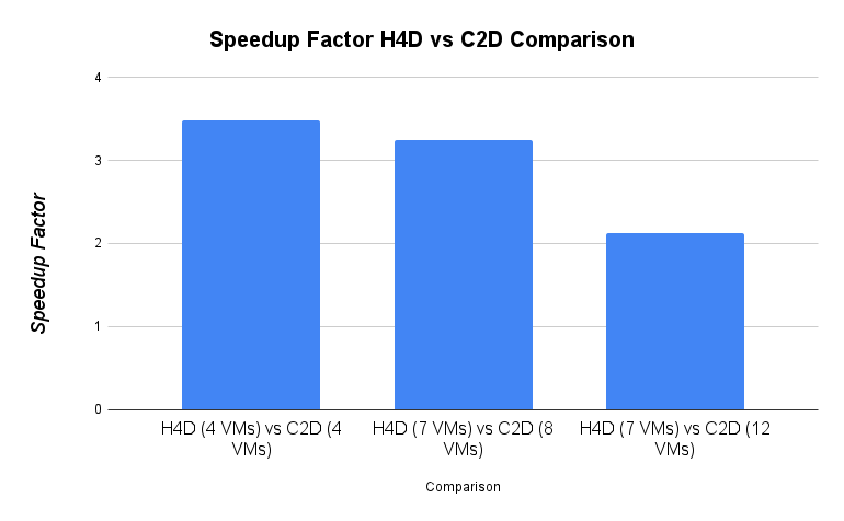
- H4D is substantially faster at scale. The H4D (7 VMs) configuration achieves the lowest average elapsed time of 0.564 seconds, which is approximately 52.9% faster than the fastest C2D configuration (1.197 seconds for C2D 12 VMs).
- For comparable scales, the H4D (4 VMs) configuration is faster (1.082 seconds) than the heavily scaled C2D (12 VMs) configuration (1.197 seconds ), representing a speed advantage of about 9.5%, despite H4D using only a third of the VMs.
Memory Consumption (Resident HWM Memory)
-
The H4D VM type uses significantly more memory, peaking at 2238.031 GB (H4D 7 VMs). However, it is important to note that it is not merely the VM type that is responsible for this higher memory usage; StarCCM+ is the application consuming more memory on this machine. The highest memory usage for H4D is approximately 304.8% higher (or about 4.05x greater) than the peak memory usage for C2D (552.646 GB for C2D 12 VMs), which has much lower memory usage, peaking at only 552.646 GB (C2D 12 VMs).
Additionally, this high water mark (HWM) remains very low compared to the total amount of memory available, which might even explain why StarCCM+ is utilizing more memory during its operations.
Speedup Comparison
- The bar plot below visualizes the calculated speedup of H4D over C2D for comparable configurations.
Conclusions
The H4D VM type demonstrates superior performance (higher throughput and lower average elapsed time) compared to the C2D VM type, especially when scaled up.
However, the C2D VM type is far more memory-efficient for this test, using approximately 4× less memory than the H4D VM type at its respective largest configurations (552.646 GB for C2D vs 2238.031 GB for H4D).
Hence, based on this benchmark, our conclusions are that the choice between H4D and C2D depends on the priority:
- Choose H4D for maximum performance and speed, particularly for tasks that can tolerate higher memory consumption.
- Choose C2D if total memory usage is a critical factor, though this comes at the cost of lower peak throughput and slightly longer execution times.
SeWaS
SeWaS is a seismic wave propagation simulator tailored for massively parallel hardware infrastructures. The application dataflow is built on top of PaRSEC, a generic task-based runtime system. In this section, we compare the performance of H4D and C2D VM types running SeWaS on a single node, focusing on execution time and parallelism. The application was built using the CMake installation procedure described in the official documentation, with Intel MPI version 2021.13.1 instead of OpenMPI for both H4D and C2D runs.
The following table summarizes the performance indicators for this test:
| Metric | H4D Value (s) | C2D Value (s) |
|---|---|---|
| Global Elapsed Time | 226.30 | 615.72 |
| Global CPU Time | 38265.44 | 33131.05 |
| Core Simulation Elapsed Time | 225.56 | 609.72 |
| ComputeVelocity Elapsed Time | 11724.35 | 10433.13 |
| ComputeStress Elapsed Time | 20964.25 | 17939.95 |
Analysis and Conclusions
Overall Execution Time
- The H4D VM type achieves a lower total execution time for the SeWaS application compared to C2D.
- Global Elapsed Time: H4D (226.30 s) compared to C2D (615.72 s).
- Speed Factor: H4D is approximately 2.72x faster than C2D.
- Time Reduction: The H4D configuration reduces the wall-clock time by 63.24% relative to C2D.
Parallelism and Resource Utilization
- The difference in overall execution time is closely correlated with the ability of each VM type to utilize its CPU resources concurrently, as indicated by the Parallelism Factor (Global CPU Time / Global Elapsed Time).
- H4D Parallelism Factor: 169.1x (38,265.44 s CPU / 226.30 s Elapsed).
- C2D Parallelism Factor: 53.8x (33,131.05 s CPU / 615.72 s Elapsed).
- Relative Utilization: H4D exhibits a 3.14x higher Parallelism Factor than C2D, suggesting a greater core/thread density or more effective parallel processing capability.
Detailed Task Analysis (Total Accumulated Time)
- When examining the total accumulated time for the primary computational tasks, the C2D VM registers slightly lower CPU time than H4D.
- ComputeVelocity Total Time: C2D (10,433.13 s) is 11.01% faster than H4D (11,724.35 s).
- ComputeStress Total Time: C2D (17,939.95 s) is 14.43% faster than H4D (20,964.25 s).
Our interpretation is that individual core efficiency of C2D may be slightly superior for these specific functions, requiring less total CPU time. However, H4D’s significant advantage in parallel execution capabilities far outweighs this minor advantage, resulting in a substantial reduction in wall-clock time.
Conclusions
The H4D VM configuration provides a significant advantage in overall wall-clock time due to its high level of parallelism. This performance difference is maintained despite C2D showing lower total accumulated CPU time for the individual core functions, confirming that H4D's capacity for high concurrency is the primary factor affecting the final elapsed time.
Chameleon
CHAMELEON is a C-based framework for solving dense linear algebra problems, including systems of linear equations and linear least squares, using factorizations like LU, Cholesky, QR, and LQ. It supports both real and complex arithmetic in single and double precision. The application was set up by following the Spack installation instructions, with the same version of Intel MPI as the previous two benchmarks. I tested the CHAMELEON DGEMM (Double-precision General Matrix Matrix Multiply) function performance on H4D VMs across varying workload sizes and node counts.
Analysis and Conclusions
Scaling by Matrix Size (1 Node Comparison)
Comparing the 1000³ matrix run to the 10000³ matrix run on a single H4D node shows a significant efficiency gain as the workload size increases.
| Configuration | Matrix Size (m, n, k) | Time (s) | GFLOPS (Performance) |
|---|---|---|---|
| 1 Node H4D | 1000³ | 0.00579 | 345.24 |
| 1 Node H4D | 10000³ | 0.4397 | 4548.37 |
Performance Increase: By increasing the matrix size from 1000³ to 10000³ (a 1000x increase in total operations), the GFLOPS figure increases from 345.24 to 4548.37. This represents a performance gain of approximately 1217% (or 13.17x), demonstrating that the H4D node is utilized far more efficiently by larger, data-intensive tasks.
Scaling by Node Count (Strong Scaling on 10000³ Matrix)
This comparison examines the effect of moving from one node to two nodes while keeping the total workload (10000³ matrix) constant.
| Configuration | Matrix Size (m, n, k) | Time (s) | GFLOPS (Performance) |
|---|---|---|---|
| 1 Node H4D | 10000³ | 0.4397 | 4548.37 |
| 2 Nodes H4D | 10000³ | 0.3103 | 6444.60 |
Time Reduction (Speedup): Increasing the node count from 1 to 2 reduces the execution time from 0.4397 s to 0.3103 s. This constitutes a time reduction of approximately 29.4%, corresponding to a speedup factor of approximately 1.42x.
Performance Scaling: The GFLOPS figure increases from 4548.37 to 6444.60, an increase of approximately 41.7%. This shows that adding a second node provides significant, though sub-linear, scaling in performance.
Scaling to Massive Workload (100000³ Matrix)
The final test examines a massive workload across 1 node versus 2 nodes.
| Configuration | Matrix Size (m, n, k) | Time (s) | GFLOPS (Performance) |
|---|---|---|---|
| 1 Node H4D | 100000³ | 278.46 | 7182.44 |
| 2 Nodes H4D | 100000³ | 131.71 | 15184.33 |
Time Reduction (Speedup): Distributing this extreme workload across 2 nodes reduces the time from 278.46 s to 131.71 s, achieving a speedup factor of 2.11x.
Efficiency: The observed speedup (2.11x) is greater than the increase in resources (2x nodes), which is typically categorized as super-linear scaling, indicating high efficiency and utilization of a multi-node H4D cluster for the most intense computational tasks.
Maximum Performance: The 2-node system achieves its highest recorded performance, 15184.33 GFLOPS (or 15.18 TFLOPS), confirming that distributing the largest, most computationally intense tasks across multiple H4D nodes maximizes the cluster's utilization and raw performance capability.
Conclusions
In summary, the data confirms that Chameleon's DGEMM routine benefits significantly from both increased workload size on a single node and effective parallel distribution across multiple H4D nodes for the most demanding problems.
Wrap Up
The performance evaluation of Simcenter StarCCM+, SeWas, and Chameleon on Google Cloud Platform highlights significant advantages of the H4D VM types over C2D VMs, particularly for high-performance computing tasks like computational fluid dynamics simulations and seismic wave propagation:
- Higher Throughput and Speed: H4D VMs demonstrated notably higher throughput and faster execution times across all tested configurations. In the LeMans-104m test case, the H4D configuration achieved a peak throughput of 132,622 Cell-Iterations per Worker-Second, representing a 15.25% increase over C2D VMs. Moreover, H4D significantly reduced average elapsed time, achieving a best time of 0.564 seconds compared to 1.197 seconds for the fastest C2D setup.
- Resource Utilization: The H4D VMs showcased superior parallelism with a Parallelism Factor of 169.1x for the SeWas application, compared to 53.8x for the C2D VMs. This demonstrates H4D's capability to maximize core utilization effectively, enhancing overall performance even in more demanding applications.
- Scaling Efficiency: The Chameleon benchmarks revealed significant performance gains as matrix sizes increased, with GFLOPS performance improving by 1217% when scaling from a 1000³ to a 10000³ matrix size. This demonstrates H4D's strong capability for handling large, data-intensive tasks, further confirmed by the remarkable speedup of 2.11x when distributing massive workloads across two nodes.
- Memory Consumption: While H4D VMs excel in performance, they come with higher memory consumption, peaking at 2238.031 GB compared to 552.646 GB for C2D VMs. This factor must be considered when selecting infrastructure, particularly in memory-constrained environments.
Final Thoughts
Choosing between H4D and C2D VMs ultimately depends on specific use cases and requirements. For applications demanding maximum computational performance and speed, H4D is the clear winner, making it ideal for high-end simulations and analyses. Conversely, for scenarios where memory efficiency is paramount, C2D VMs remain a competent choice, albeit at the expense of lower throughput and longer execution times.
Overall, these benchmarks provide critical insights for organizations looking to leverage cloud-based HPC solutions, enabling informed decisions tailored to their computational needs. Considering the performance improvements observed, I encourage you to benchmark your workloads and see these improvements by yourself.